Machine Learning Optimization - Variance Reduction Techniques | Alex Salce

Table of Contents
0: Introduction
1: Crash Course: Gradient Descent
2: Stochastic Gradient Descent
4: SARAH and ADAM Algorithms

Variance Reduction Techniques

The Bias-Variance Tradeoff

You may already be familiar with a bias-variance tradeoff scenario in machine learning -- our model is not producing desirable training error, so we choose to increase the complexity to better fit the training data. However, in doing so we may find that we "overfit" the model to the training data and create a prediction model that is biased to the details and minutae of the training data. When we apply the model to test data that it has not previously seen, it performs more poorly than our simpler model.

This is commonly referred to as "overfitting" and is an example of a biased model. As we increase the complexity of our model, we are trading the magnitude of prediction error to the test data (variance) for bias to the training data itself.

The bias-variance tradeoff we see in variance reduction techniques for SGD algorithms is fundamentally different than our familiar example.

Model complexity bias-variance tradeoffs can affect the error in predictions by the model itself -- but in the context of stochastic optimizaiton, bias and variance can impact error in parameter updates.

The issue with this variance in general ends up being the rate at which we converge, or whether we converge at all. Variance that overwhelms the steps, it can adversely impact the rate at which we converge to an acceptable solution, and if our algorithm takes too long to execute, we have defeated the purpose of using stochastic methods. In all, our goal becomes finding a balance of the computational advantages of stochastic processes while keeping variance (and as we will see, bias) under control in order to reap the advantages of faster algorithms.

NOTE

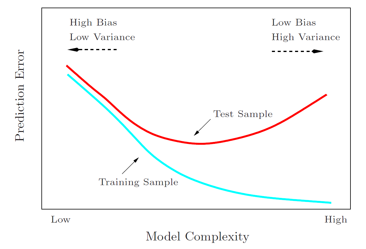
p.38, a general illustration of the bias-variance tradeoff

MSE, Variance and Bias

Before we get into some techniques that can address variance in stochastic descent, we need to observe one of the core principles of statistical anlysis.

Part of our due diligence in statistics is to analyze the quality of an esimator. To quantify the accuracy of an estimator $\hat{\boldsymbol{\theta}}$ , we measure the error of the estimator compared to the true value of the parameter $\boldsymbol{\theta}$ it is estimating by using Mean Squared Error (MSE).

MSE is a quantity defined as the expected value of the square difference between the parameter estimate and the true parameter value. Skipping some steps in between, it can be decomposed into both a variance component and a bias component (a link to a helpful video about MSE).

\begin{aligned} \text{MSE}(\hat{\boldsymbol{\theta}}) = \mathbb{E}_{\theta}[(\hat{\boldsymbol{\theta}}-\boldsymbol{\theta})^2] = \text{Bias}(\hat{\boldsymbol{\theta}})^2 + \text{Var}(\hat{\boldsymbol{\theta}}) \end{aligned}

In statistics, we often measure the quality of an estimator by whether it is both unbiased and consistent. We won't dive into consistency of estimators further here (see appendix for some detail), but we do want to take note that in general, unbiased estimators are preferred estimators to those that are biased in some way. In terms of MSE, if our estimator is unbiased, then its MSE is equal to its variance.

In the previous section some examples of an unbiased estimator.

For example, we assume our conditional estimator of the approximation error for a gradient, $\boldsymbol{w_{k}} | \boldsymbol{\theta_{k}}$ is unbiased, i.e. $\mathbb{E} [\boldsymbol{w_{k}} | \boldsymbol{\theta_{k}}] = 0$ , where $\boldsymbol{w_{k}} \overset{\Delta}{=} \nabla f(\boldsymbol{\theta_{k}}) - \nabla f_{i_{k}}(\boldsymbol{\theta_{k}})$ . So, the MSE for the estimator $\boldsymbol{w_{k}} | \boldsymbol{\theta_{k}}$ is only its variance.

We showed $\text{Var}(\boldsymbol{w_{k}} | \boldsymbol{\theta_{k}}) = \mathbb{E} [\boldsymbol{w_{k}} \boldsymbol{w_{k}}^T | \boldsymbol{\theta_{k}}] \leq \mathbb{E} [||\boldsymbol{w_{k}}||^2 | \boldsymbol{\theta_{k}}]$ , so the MSE of $\boldsymbol{w_{k}} | \boldsymbol{\theta_{k}}$ , the estimate of stochastic gradient estimation error for a given $\boldsymbol{\theta_{k}}$ , is the following.

\begin{aligned} \text{MSE}(\boldsymbol{w_{k}} | \boldsymbol{\theta_{k}}) = \mathbb{E} [\boldsymbol{w_{k}} \boldsymbol{w_{k}}^T | \boldsymbol{\theta_{k}}] \end{aligned}

which is bounded by a constant variance term.

\begin{aligned} || \text{MSE}(\boldsymbol{w_{k}} | \boldsymbol{\theta_{k}}) || \leq \sigma^2 \end{aligned}

It is important to be cognizant of MSE as the measure for error of an estimator rather than just the variance. We don't just care about variance -- bias is a nontrivial and undesirable quantity if we are not careful.

As we explore variance reduction techniques, we will see that if we attempt to curb error due to variance but do not reduce overall MSE of the estimator in doing so, that MSE information is only "transferred" to the bias component. Compounding effects of bias in recursive descent algorithms can become especially problematic, so as we continue, we will give special attention to ensuring we also take it into account.

Minibatch SGD

Since variance in the algorithm's steps is a consequence of using estimates of the full gradient, it is pragmatic to utilize improved approximations. One natural statistical approach to improving an approximation is simple, we should use more data. We can do so by taking random batch samples of the full data -- minibatches.

Minibatches are an important variance-reduction technique that are commonly seen in the class of gradient descent algorithms. Rather than sampling random individual gradients from the full gradient at each step, we can improve our gradient approximation by sampling a random subset $I_k \subset \{ 1,...,n \}$ where $|I_k|=b < < n$ and modify the SGD algorithm to average the "minibatches".

\begin{aligned} \boldsymbol{\theta}_{k+1}=\boldsymbol{\theta}_{k}- \frac{\alpha_{k}}{b} \underset{i \in I_k}{\sum} \nabla f_{i_{k}}(\boldsymbol{\theta}_{k}) \end{aligned}

See appendix for example calculation details

We first take the conditional expectation modified from SGD. Note, as with SGD the gradient estimate is unbiased $E[\frac{1}{b} \underset{i \in I_k}{\sum} \nabla f_{i_{k}}(\boldsymbol{\theta}_{k})] = \nabla f(\boldsymbol{\theta}_{k})$ .

\begin{aligned} || \text{MSE}(\boldsymbol{w_{k}} | \boldsymbol{\theta_{k}}) || = \mathbb{E}[||\boldsymbol{w_k}||^2 | \boldsymbol{\theta_k}] = \mathbb{E}[|| \frac{1}{b} \underset{i \in I_k}{\sum} (\nabla f_{i_{k}}(\boldsymbol{\theta}_{k}) - \nabla f(\boldsymbol{\theta}_{k})) ||^2 | \boldsymbol{\theta_k}] \end{aligned}

\begin{aligned} \leq \frac{1}{b^2} \cdot b \underset{i \in I_k}{\sum} \mathbb{E}[ || (\nabla f_{i_{k}}(\boldsymbol{\theta}_{k}) - \nabla f(\boldsymbol{\theta}_{k})) ||^2 | \boldsymbol{\theta_k} ] \leq \frac{\sigma^2}{b} \end{aligned}

NOTE

The above calculation uses the identity $||\overset{n}{\underset{i=1}{\sum}} a_i||^2 \leq \overset{n}{\underset{i=1}{\sum}} ||a_i||^2$ to derive inequality.*

We can reduce the variance bound by a factor of batch size be $b$ . Since the estimator is unbiased, we do not need to be concerned with mere displacement of MSE a bias term. Intuitively we can make sense of this since we are using more information for each gradient calculation, and thus we get a better approximation $\nabla f_{i_{k}}(\boldsymbol{\theta}_{k})$ of the gradient $\nabla f(\boldsymbol{\theta}_{k})$ at each step $k$ . Note here also that this result does not require a diminishing learning rate, so it can be applied to gradient descent algorithms with constant or adaptive learning rates.

The tradeoff here, though, is a more expensive gradient computation by a factor of $b$ at each timestep. No free lunch! A convergence analysis will show that minibatch SGD converges at a rate $\mathcal{O}(\frac{1}{\sqrt{T}})$ , which is the same as SGD but at greater expense computationally due to the batch size. It's largely considered a compromise between SGD and regular gradient descent.

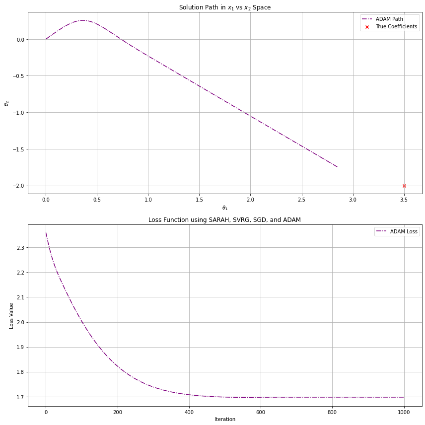
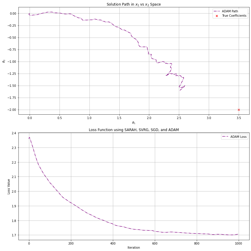
The ADAM optimizer, which we will see in greater detail later, utilizes batch gradients. We are fitting to the same correlated noise data from above, which has $n=100$ samples and two features $\theta_1$ and $\theta_2$ . The above graphs demonstrate the effects of variance reduction for increasing batch sizes. The first plot uses a batch size of $b=100$ (which is essentially regular gradient descent with ADAM's boost), the second $b=10$ , and the last $b=2$ . Clearly, we get closest to our optimal solution using bigger batches to reduce variance in the steps, but what this does not capture is additional computational cost for each step. Ultimately, we tune parameters like batch size to find a balance between performance and results.

Stochastic Average Gradient (SAG) and SAGA

SAG and SAGA utilize important variance reduction techniques and are often treated as benchmarks for comparison with stochastic and batch gradient descent algorithms. Minibatches serve well in reducing variance, however as we increase the batch size, we are also increasing the per-iteration computational cost; as $b$ approaches $n$ , we end up back where we started with regular gradient descent. Our goal is to achieve a convergence rate of $\mathcal{O}(\frac{1}{T})$ with a cost of one gradient per iteration, motivating SAG.

Stochastic Average Gradient (SAG)

The framework for SAG uses gradient descent in the following form, taking the average gradient at each iteration.

\begin{aligned} \boldsymbol{\theta}_{k+1}=\boldsymbol{\theta}_{k}- \frac{\alpha}{n} \sum_{i=1}^{n}{g_k^{(i)}} \end{aligned}

where $g_k^{(i)} = \nabla f_i(\boldsymbol{\theta}_{k})$ .

For SAG, we will update only one gradient at step $k$ , $g_k^{(i_k)} = \nabla f_{i_k}(\boldsymbol{\theta}_{k})$ for uniformly random chosen $i_k$ , and keep all other $g_k^{(i)}$ at their previous value.

To accomplish this, the procedure maintains a table containing $g_k^{(i)}(\boldsymbol{\theta}) = \nabla f_{i}(\boldsymbol{\theta})$ , $i=1,...,n$ . This table does require additional storage computationally proportional to the size of the data.

We first initialize $\boldsymbol{\theta}_{0}$ and set $g=0$ and $g^{(i)}=0$ for all $i=1,...,n$ .

At each step $k=1,2,3...$ we select $i_k \in \{1,...,n \}$ uniformly at random and update our individual gradient, keeping all other values of $g_k^{(i)}$ the same.

\begin{aligned} g_{k}^{(i)} = \begin{cases} \nabla f_{i}(\boldsymbol{\theta}_{k-1}) & i=k\\ g_{k-1}^{(i)} & i\neq i_{k} \end{cases} \end{aligned}

We then perform the per iteration update.

\begin{aligned} \boldsymbol{\theta}_{k}=\boldsymbol{\theta}_{k-1}- \alpha \left ( \frac{1}{n} \sum_{i=1}^{n}{g_k^{(i)}} \right ) \end{aligned}

We now have a new estimator for the gradient which we will call $\hat{g}$ , which can be written as the following.

\begin{aligned} \hat{g} = \frac{1}{n} \left( g_k^{(i_k)} - g_{k-1}^{(i_k)} \right) + \frac{1}{n} \sum_{i=1}^{n}{g_{k-1}^{(i)}} \end{aligned}

If we set $X = g_{k}^{(i_k)}$ and $Y = g_{k-1}^{(i_k)}$ , noting that $\mathbb{E}[Y] = \frac{1}{n} \overset{n}{\underset{i=1}{\sum}}{g_{k-1}^{(i)}}$ , $\hat{g}$ can be rewritten as the following.

\begin{aligned} \hat{g} = \frac{1}{n} \left( X - Y \right) + \mathbb{E}[Y] \end{aligned}

As with our previous analysis of estimators, we take the expectation of $\hat{g}$ ,

\begin{aligned} \mathbb{E}[\hat{g}] = \frac{1}{n} \left( \mathbb{E}[X] - \mathbb{E}[Y] \right) + \mathbb{E}[Y] \end{aligned}

\begin{aligned} = \frac{1}{n} \mathbb{E}[X] - (1-\frac{1}{n})\mathbb{E}[Y] \neq 0 \end{aligned}

Our expectation for our estimator is nonzero, so our gradient estimator $\hat{g}$ is biased!

Omitting the details, SAG can be shown to converge under our usual convexity and Lipschitz continuity for the gradient per the following. For $\alpha = \frac{1}{16L}$ and and the intialization,

\begin{aligned} g_{0}^{(i)} = \nabla f_i(\boldsymbol{\theta}_{0}) - \nabla f(\boldsymbol{\theta}_{0}) \text{, } i=1,...,n \end{aligned}

we achieve the following convergence.

\begin{aligned} \mathbb{E}[f(\bar{\boldsymbol{\theta}}_T)-f(\boldsymbol{\theta}^*)] \leq \frac{48n}{T} \left( f(\boldsymbol{\theta_0}) - f(\boldsymbol{\theta^*}) \right) + \frac{128L}{T}|| \boldsymbol{\theta_0} - \boldsymbol{\theta^*} ||^2 \end{aligned}

Comparing directly to SGD:

This is the desired $\mathcal{O}(\frac{1}{T})$ (more accurately $\mathcal{O}(\frac{n+L}{T})$ ), which is overall an improvement as compared to SGD $\mathcal{O}(\frac{1}{\sqrt{T}})$
Converges with constant learning rate
SAG does not require the assumption of conditional boundedness of the variance ( $\mathbb{E}[ || w_k ||^2 | \boldsymbol{\theta_k} ] \leq \sigma^2$ )
BUT this algorithm is biased
It's a drawback computationally to need to store a gradient table

SAGA

The SAGA algorithm is only a slightly modified version of SAG, with the only difference being a modification of the gradient estimate itself. We will still maintain our table of gradients, use the same initialization procedure, and pick/replace a random gradient in the same fashion.

Instead, however, of the SAG gradient estimate $\hat{g} = \frac{1}{n} \left( g_k^{(i_k)} - g_{k-1}^{(i_k)} \right) + \frac{1}{n} \sum_{i=1}^{n}{g_{k-1}^{(i)}}$ , we use the following gradient estimate for SAGA.

\begin{aligned} \hat{g} = g_k^{(i_k)} - g_{k-1}^{(i_k)} + \frac{1}{n} \sum_{i=1}^{n}{g_{k-1}^{(i)}} \end{aligned}

So, our per iteration updates are of the following form.

\begin{aligned} \boldsymbol{\theta}_{k}=\boldsymbol{\theta}_{k-1}- \alpha \left ( g_k^{(i_k)} - g_{k-1}^{(i_k)} + \frac{1}{n} \sum_{i=1}^{n}{g_k^{(i)}} \right ) \end{aligned}

SAGA can be shown to have the same convergence $\mathcal{O}(\frac{1}{T})$ , but can use a slightly better learning rate $\alpha = \frac{1}{3L}$ . It also does not require the bound on conditional variance. The most stark difference with SAGA vs. SAG is that SAGA is unbiased. It still has the less than desirable need to store a gradient table.

Using the same definition for random varables $X$ and $Y$ as before, we have the following.

\begin{aligned} E[\hat{g}] = E[X] - E[Y] + E[Y] = E[X] = \nabla f(\boldsymbol{\theta_k}) \end{aligned}

So, $\hat{g}$ is an unbiased estimator for the gradient and it follows that the bias term $E[w_k | \boldsymbol{\theta}_{k}] = 0$ for this method.

SAG & SAGA Variance comparison

Recall the gradient estimates for each.

SAG

\begin{aligned} \hat{g} = \frac{1}{n} \left( g_k^{(i_k)} - g_{k-1}^{(i_k)} \right) + \frac{1}{n} \sum_{i=1}^{n}{g_{k-1}^{(i)}} \end{aligned}

SAGA

\begin{aligned} \hat{g} = g_k^{(i_k)} - g_{k-1}^{(i_k)} + \frac{1}{n} \sum_{i=1}^{n}{g_{k-1}^{(i)}} \end{aligned}

For $X = g_{k}^{(i_k)}$ and $Y = g_{k-1}^{(i_k)}$ where $X$ and $Y$ are correlated, we have the general form.

\begin{aligned} \hat{g}_{\alpha} = \alpha (X-Y) + \mathbb{E}[Y] \end{aligned}

Where $\alpha = 1$ for SAGA and $\alpha = \frac{1}{n}$ for SAG.

Taking the variance, we have the following.

\begin{aligned} Var(\hat{g}_{\alpha}) = \alpha^2 (Var[X] + Var[Y] - 2 Cov[X,Y]) \end{aligned}

So, we can compare the methods.

\begin{aligned} \textbf{SAG: }Var(\hat{g}_{\alpha}) = \frac{1}{n^2} (Var[X] + Var[Y] - 2 Cov[X,Y]) \end{aligned}

\begin{aligned} \textbf{SAGA: }Var(\hat{g}_{\alpha}) = (Var[X] + Var[Y] - 2 Cov[X,Y]) \end{aligned}

SAGA's modified algorithm makes the iterations unbiased, however by doing so we increase variance in the steps. The SAG/SAGA has tradeoffs with bias and variance, but ultimately both converge at the same rate. In terms of MSE, this means we may not have an obvious advantage for either method other than the faster learning rate of SAGA.

Other Common Variance Reduction Techniques

We have covered some basics of stochastic gradient descent algortihms, as well as some basic approaches to variance reduction, but I also wanted to include some supplemental material for further reading on the basics of the topics. If you are interested in learning more about some common techniques, I recommend this paper on variance reduction techniques in machine learning (Gower et al., 2020).

Next: SARAH and ADAM Algorithms

Gower, R. M., Schmidt, M., Bach, F., & Richtarik, P. (2020). Variance-Reduced Methods for Machine Learning. https://arxiv.org/abs/2010.00892