SARAH
SARAH, or StochAstic Recursive grAdient algoritHm, is a stochastic gradient descent method that utilizes recursive gradient information to reduce variance in the steps. The algorithm is a modification of the method SVRG (Stochastic Variance Reduced Gradient), which we will briefly cover, and is widely used as one of the benchmark algorithms for comparison to new gradient descent style methods. As with other methods we have seen until now, some of its core assumptions for convergence require a convex objective function (or strongly-convex) with Lipschitz continuous gradient. SARAH is a good example of an algorithm that is actually biased, but can be an improvement over SVRG if conditions are considered carefully.
Stochastic Variance Reduced Gradient (SVRG)
To understand the SARAH algorithm, we need to first conceptually understand SVRG. First, we present the SVRG algorithm.

The algorithm consists of an outer loop and an inner loop, both with iterations specified as hyperparameters. We select the number of epochs (each "epoch" is one pass over all samples in the dataset) for the outer loop, and the number of inner loop iterations .
The outer loop performs one full gradient computation using the initialized parameter , which begins with the initialized parameter that is used to make one full gradient computation (hence outer loop "epochs"). is then used to initialize the inner loop updates , and fed into the loop with .
The inner loop then begins, using a stochastic gradient approach in combination with an iteratively updated gradient estimate , utilizing the outer loop full gradient , the stochastic gradient computed from the most recent parameter update , and the corresponding full-gradient sample . The gradient estimate is then used for a normal gradient descent style parameter update.
All parameter updates occur within the inner loop, and the resulting parameters from the inner loop get fed back into the outer loop as the new parameter initialization.
SVRG Gradient Estimator
We want to analyze our gradient estimate, so we take its expectation conditioned on knowledge of .
So, the SVRG gradient estimator for the inner loop updates is unbiased.
SVRG Variance Reduction
The variance reduction for SVRG is accomplished with the inner loops by the convergence of both and to the same optimal parameter . Omitting the detailed proof (Johnson & Zhang, 2013) (link), the following holds for convex (and strongly convex) objective functions with Lipschitz continuous gradients.
So if , then
This means that the variance of the gradient estimates approach zero as the parameter updates converge to the optimum , hence the inner loops serve as a variance reduction technique, but in order for overall variance in the steps to decrease we must update (so that ), meaning that we must execute additional full gradient computations (epochs). We will revisit this point in the analysis of the variance reduction of SARAH.
SVRG Convergence
For convex and Lipschitz continuous gradient objective functions , SVRG can be shown to converge at a rate of , which is an improvement over SGD's . It also has better theoretical convergence, , than SAG and SAGA, () (note convergence here is in terms of specified tolerance rather than number of iterations ).
For a -strongly convex objective function, SVRG converges to the following.
Assume is sufficiently large such that the following holds.
then,
The complexity is , which is comparable to SAG/SAGA. This also gives us criteria for which to select inner loop size and learning rate .
Unlike SGD, we do not need a decaying learning rate for SVRG to achieve the comparable convergence rate. The decaying learning rate required for SGD is a consequence of the variance in the steps (even though variance can be unbounded), which is a good example of how variance can impact convergence rate; SVRG explicitly reduces the variance in the steps of SGD.
The SARAH Algorithm
Methodology in this section is drawn from SARAH: A Novel Method for Machine Learning Problems Using Stochastic Recursive Gradient (Nguyen et al., 2017) (link)
(Nguyen, Liu, Scheinberg, and Takáč, 2017)

SARAH is very closely related to SVRG. It utilizes the same outer/inner loop apprach that functionally serve the same purpose; the outer loop is used to compute a full gradient (a "snapshot" of the full gradient), and the inner loop performs SGD style steps with a variance reduction design. The key difference between SVRG and SARAH is in the gradient estimate update step in the inner loop.
SVRG's gradient estimate is designed to use the outer loop "snapshot" to generate an unbiased gradient estimate at each step, while simultaneously reducing the variance that is a consequence of SGD. The "snapshot" is what stablizes the algorithm in terms of bias (the gradient estimate is unbiased) and allows the variance in the stochastic steps to be reduced using the parameters from which the outer loop was initialized.
SARAH's gradient estimate, however, leans more heavily into the variance-reduction aspect of the algorithm by utilizing recursive gradient information to reduce variance, rather than solely using the gradient estimate from the outer loops. This improves the stochastic variance reduction power of the algorithm, but at the expense of introducing bias.
SARAH Gradient Estimator
The gradient estimate (also referred to as the "SARAH update") utilizes a similar framework to SVRG. Recall the SVRG gradient estimate.
The SARAH estimator modifies the gradient estimate by replacing the gradient esimate terms from the outer loop initialization with a recursive gradient update.
We note that there is a shift in index as we now need to use both the most recent random gradient as well as the random gradient from the previous step. This also means that we must perform one parameter update in the outer loop before we enter the inner loop.
Each gradient estimate uses every previous gradient estimate from the inner loop for each inner loop update, hence a "recursive" update framework as opposed to each update using the outer loop initialization only.
Let's take the conditional expectation of the gradient estimate, given all previous iterates of . We will call this , the -algebra generated by the inital and all subsequent randomly chosen indices for the inner loop . Note that .
The steps are omitted, but the result is notable as it is not an unbiased estimator for the gradient. However, the total expectation holds.
So, an exact full pass over the data for an inner loop is unbiased.
SARAH Variance Reduction
Recall for SVRG that in order for overall variance in the steps to reduce, we must execute additional outer loops; in order for to hold, we must update via an outer loop computation.
In the analysis of SVRG we showed that stochastic gradients are unbiased estimators for the full gradient, and that . Since the inner loop terms only utilize stochastic gradients for the gradient estimate, the inner loops will reduce variance without requiring an outer loop as there are no terms in the estimator dependent upon the outer loop update.
SARAH's variance bound in the -strongly convex objective function case can be shown to be less than the variance bound of the same objective function with SVRG.
The variance reduction of the inner loops is at the expense of bias; SARAH reduces variance in the inner loops but now has bias that is itself stochastic. This bias can be somewhat "corrected" for, however, by executing an outer loop to reinitialize the parameters by pointing them in the correct direction. We will examine some intelligent ways to execute outer loops when necessary using SARAH+.
SARAH Convergence
For convex and Lipschitz continuous gradient objective functions , SARAH can be shown to converge at a rate of . Better conditioned s that are -strongly convex converge at a rate of .
Comparing these rates directly to SVRG,
| Convexity | SVRG | SARAH |
|---|---|---|
| Convex | ||
| Strong Convexity |
Similar to SVRG, we must select our inner loop size and learning rate such that the following holds.
Recall from above that the variance bound for SARAH in the strongly convex case is smaller than that of SVRG. So, while their convergence complexity is the same for strong convexity, SARAH can use a larger learning rate than SVRG. SVRG must use a learning rate of whereas SARAH can use .
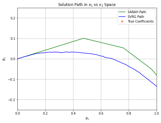
We revisit a side by side comparison of SARAH and SVRG, both run with the same number of inner and outer loops with the same hyperparameter settings. The first image is zoomed in to highlight how each algorithm handles variance reduction. SARAH has very little variance, but requires outer loop executions to correct for its inner loop bias (outer loops happen at the "kinks"). SVRG starts moving toward the solution sooner, but has higher variance in its steps until we execute more outer loops, and it smooths as more outer loops are executed (our gradient estimate becomes better). In the same number of iterations, however, they are fairly comparable. This is only a very simple example to illustrate their general behaviors, but reinforces that they are very similar algorithms in nature and performance. So, there are some advantages to SARAH over SVRG, but not necessarily overwhelmingly so.
SARAH+ Algorithm

Nguyen et al. (2017) (link) present this variant of the SARAH algorithm that provides an automatic and adaptive inner loop size. Numerical experiments from the paper indicate a selection of shows benefits in rate for their numerical experiments, but does not elaborate on any theory.
This modification introduces an automated methodology for breaking the inner loop such that inner loop size can be adaptive. It also serves as automation to correct for bias in the inner loops with the execution of a full outer loop gradient.
Applications of SARAH
In practice, SARAH can be a direct substitute for SVRG with only some updated parameter tuning considerations, so it can be utilized for a very large variety of applications as a SVRG replacement. However, it does not seem to be used as widely in practice as SVRG. While speculation as to why is not worthwhile, it is noteworthy that SARAH's variance reduction technique utilizes a biased methodology, where SVRG is unbiased. SVRG is a widely utilized benchmark algorithm, and many machine learning packages have SVRG built in; the same cannot be said for SARAH, and while it does have theoretical advantages, it does not seem to have penetrated the infrastructure of optimization algorithms in practice. Still, there is a fair amount of research available for futher modifications of SARAH.
ADAM
Methodology in this section is drawn from Adam: A Method for Stochastic Optimization (Kingma & Ba, 2017) (link).
ADAM is a widely popular optimizer in machine learning. It is a staple for deep learning, neural networks, natural language processing, and generative adversarial networks applications, to name a few. ADAM has some unique strengths against other optimizers; it is fast, requires little hyperparameter tuning, performs well with sparse gradients, and can be applied to stochastic objective functions. It is also an adaptive algorithm that uses adaptive step sizes according to data it has seen to speed up convergence.
The ADAM optimizer is a stochastic/batch gradient descent variant that utilizes two techniques that leverage previous gradient information (conceptually adjacent to recursion we saw in SARAH), Momentum and RMSProp (Root Mean Squared Propogation). Momentum acts to dampen oscillations by using previous gradient moving averages to decrease the variance in steps. RMSProp adaptively scales the learning rate based upon an exponential weighted average of the magnitude of recent gradients, so it can "speed up" and "slow down" such that it does not diverge from the local data. Additionally, ADAM can utilize batch gradients rather than only individual stochastic gradients, which can act as variance reduction by increasing sample size.
The Algorithm

NOTE
is equivalent to element-wise multiplication of gradients
Variance Reduction
Momentum
Polyak's momentum is a technique that uses both the current gradient as well as the history of gradients in previous steps to accelerate convergence. The momentum term is incorporated in general with gradient descent style algorithm and uses a hyperparameter to scale its weight.
If we expand this term,
If these recent gradients are similar, the algorithm gets an additional "boost", or "momentum". and so on can be expanded similarly, and we get higher order terms as the algorithm iterates. This favors the most recent gradients since and higher order terms quickly dampen out previous iterates.
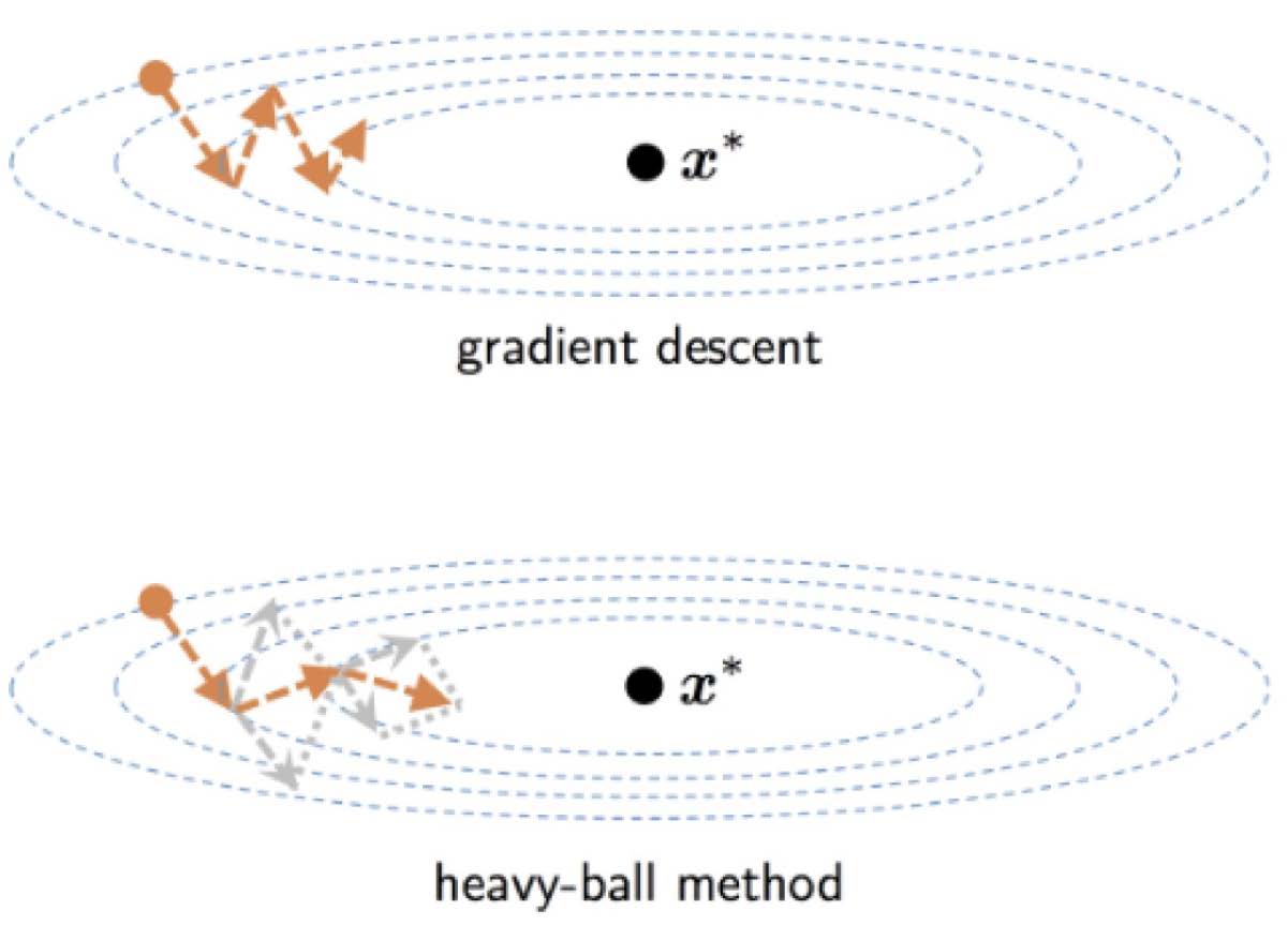
We see the "boost" in the animation for the ADAM algorithm compared to other stochastic methods, moving more rapidly toward the solution.
In ADAM, the momentum term is written as follows.
Momentum helps to accelerate convergence, particularly over the contours of objective functions, while also acting as variance reduction in the steps. The technical details of variance reduction in stochastic methods are a little more involved and are covered in (Arnold et al., 2019) (link). For and in-depth and beautifully interactive blog about momentum, I also suggest this post.
Minibatches
Earlier in this post we covered the variance reduction properties of using stochastic minibatches for variance reduction in the steps. ADAM utilizes minibatches, and the batch size is a tuneable hyperparameter. This gives us the ability to use better gradient approximations for our steps and balance convergence with computation time.
RMSProp
Root-mean-squared propograaion (RMSProp) is a technique that uses the moving average of the magnitude of recent squared gradients to normalize the gradient estimate in the descent algorithm. Its implementation in descent algorithms makes the learning rate adaptive to the data, rather than treating it as a constant tuneable hyperparameter. In essence, the learning rate will speed up or slow down depending on recent gradients.
The RMSProp update is similar to momentum, using the squared gradient term.
And the update rule in a gradient descent algorithm is written as follows.
The term only serves to stablize the algorithm as becomes small (the steps will become large if the denominator is small), preventing overshooting close to the optimum.
Bias and Bias Correction
The bias-correction steps in ADAM are enhancements to the momentum and RMSProp algorithms (which are themselves biased) and can be attributed to its advantageous performance with sparse data. ADAM is biased toward its initialization, which in general should be chosen to be the vector.
We will follow the derivation of the bias terms as in Kingma & Ba (2017)
Our momentum term , or the first moment estimator, is meant to estimate the gradient , so we want to find the expectation of the first moment estimate .
Let's first consider running ADAM for timesteps, and let be the gradients at each timestep. We assume the gradients are distributed as . At timestep , the first moment estimate term is the following.
We initialize the first moment weights setting and expand this term by substituting with each previous timestep, we get
Now, we can then take the expectation of .
We can rewrite by adding and subtracting , giving , giving the following.
Recent gradients will be close to , and gradients further in the past will be quickly dampened by as it should be selected to be small, so the term can be treated as small. So, our expectation can be written as the following.
Expanding the sum and cancellations of term results in the following.
The calculation steps for the second moment estimates follow identical logic, and we get the following expectation for .
Clearly, is a biased estimator for , and is biased for .
We can approximately correct for bias in each term by assuming initialization of moments to be zero, and by dividing the respective estimates by the and term for the first and second moment estimates respectively, giving approximately and .
ADAM Convergence
ADAM requires only a basic convexity assumption of the objective function, and a similar but more relaxed assumption of Lipschitz continuity called smoothness (Wang et al., 2022) (link). Foregoing the details, ADAM converges at a rate of (the detailed proof for ADAM's convergence can be found in original paper).
Recall that this is the same theoretical convergence rate as SGD, however it is able to used a fixed learning rate rather than a diminishing step size. While its rate is less desirable than other algorithms we have seen, it is still a widely desirable algorithm for it's performance in practice.
Applications of ADAM
ADAM is a very widely used optimizer, particularly for neural network, deep learning, and natural language processing applications amongst others. One of its advantages is how well it handles sparse data, which are commonly characteristic of the data for these types of tasks. While it is not the fastest method in terms of convergence, the methodologies it utilizes to balance stochasic variance while also addressing inherent estimator bias, making this method a trustworthy workhorse.
There is existing infrastructure for ADAM among some common machine learning tools like Keras, scikit-learn, PyTorch, and TensorFlow, to name some prolific packages in industry and research applications, so it has been embraced by the community as an effective optimizer. Overall it is a robust optimizer with reliable performance for convex (as well as nonconvex, He et al. (2023)) objectives.
Example Numerical Experiments
NOTE
This section was lifted directly from my coursework. Note this section uses for the model parameter vector instead of the we have been using previously (different choices may be seen in practice).
The purpose of the numerical experiment will be to evaluate general performance of ADAM and SARAH on real data and to illustrate a bias-variance tradeoff between SVRG and SARAH. We use the "Wine Quality" dataset from the UC Irvine Machine Learning Repository (Cortez et al., 2009). The data are measurements of wine characteristics (features) used to predict wine quality scores. There are instances and features. The experiements will use a simple least squares linear regression objective, assuming a system with data and response is of the form .
The least squares objective was chosen because it is strongly convex. was computed separately using scipy.optimize.lsq_linear with tolerance set to .
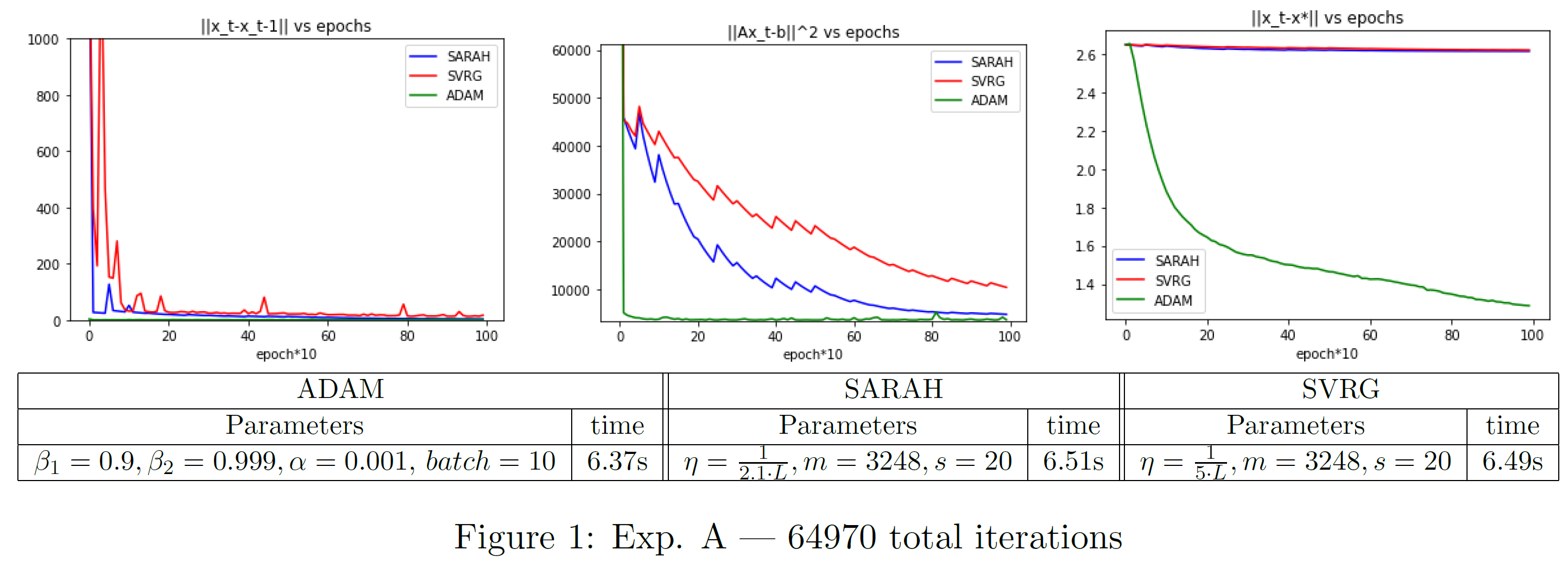
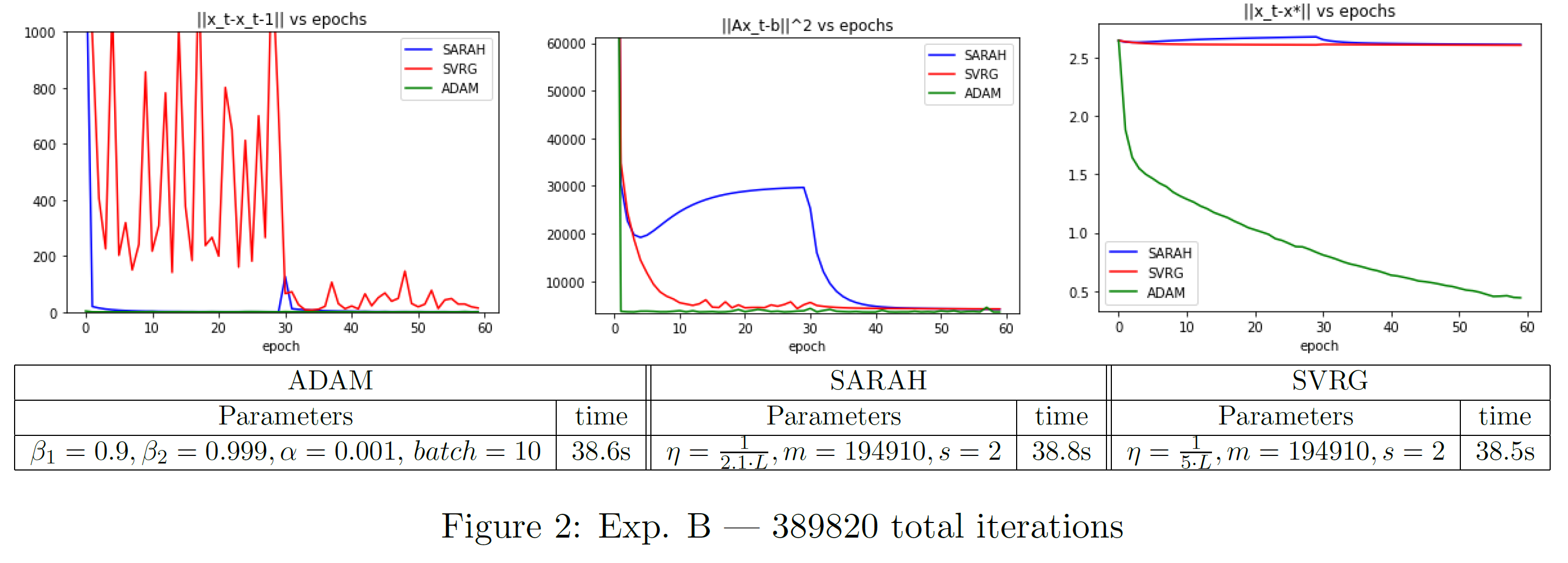
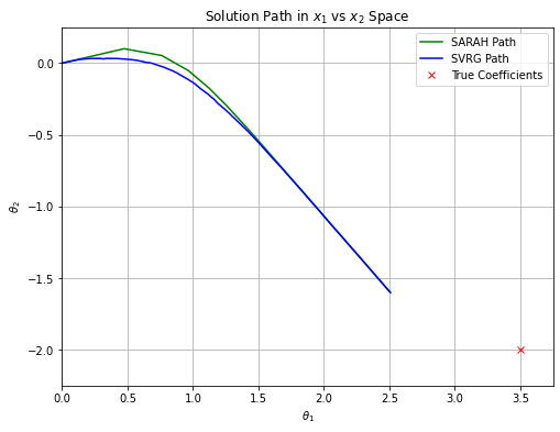
See Figures 1 and 2 for settings and computation time. The two examples chosen illustrate some high level takeaways. In terms of per-iteration computational performance, both ADAM and SARAH are virtually identical to SVRG, though ADAM can become slightly slower for increased batch sizes. SARAH and SVRG are limited in flexibility for learning rate with this data since is large and learning rate is . Both are descending, but are moving extremely slowly toward , and the larger learning rate for SARAH hardly presents an advantage. We can see benefit of the adaptive learning rate of ADAM for both Exp A and B; it is moving toward it much faster and it continues to descend as iterations increase ( vs. epochs).
Comparing SARAH and SVRG, we run the inner loop for half an epoch in Exp. A and for 30 epochs in Exp. B. The parameter choice in Exp. B adheres with SARAH's variance bound requirement . Note that for this data, the iterations required for an accurate convergence with SARAH, for a reasonable choice of , was prohibitive. In both Exp. A and B, is clearly smoother for SARAH than SVRG, however we observe that the number of effective passes over the data in the inner loop can matter. In both the and plots, SARAH will stray away from the optimal solution due to bias after around 4 epochs. It is ultimately corrected by the second outer loop step, but we can see how the biased steps of the inner loop can cause SARAH drift, whereas SVRG continues to descend. As is the reality of statistics, we are trading variance for bias.