GitHub Repo

Note: This is an adaptation of a collaborative project with contributions from Matthew Wallace and Raymond Owino

Introduction

Wildfire incidence data describes the spatial origin of a wildfire and its resulting size, which lends itself well to be studied by methods in spatial statistical analyses. Spatial statistical models can be valuable in real applications for wildfire prevention, giving inferential insights into wildfire risk as well as tools to aid in resource allocation for mitigation efforts and planning. This project seeks to build models that could be useful for these kinds of efforts, and the research questions aim to provide insight to what kinds of environmental and human factors can influence the size of a resulting wildfire based upon where it originates spatially.

Wildfire Incidence Data

Accompanying this post in the Github repo is wfigs_az_sf_EPSG32612.RData which imports wfigs_az_sf to the R environment, an sf object with 18089 observations of wildfire incidence in the state of Arizona as well as corresponding covariate data for each entry. This data was originally acquired via Wildland Fire Incident Locations from the National Interagency Fire Center. It contains spatial point data indicating the origin of each wildfire recorded in the IRWIN database (since 2014), and includes many useful data attributes for each entry. The attributes from this dataset that we used were the following.

• x and y | Spatial coordinates in lat/lon
• IncidentSize | Size of the resulting wildfire in acres
• FireCause | Human, Natural, Unknown, Undetermined
• FireDiscoveryDateTime | Date & time of incident reporting
• IncidentTypeCategory | WF (wildfire) or RX (prescribed burn)

Additional covariate data that was captured for each incidence point will be discussed later in the report.

Research Questions

Our research questions were driven by our curiosities about the ways in which we could approach modeling the data. We were also motivated in part by our findings during our explorations, and we wanted to evaluate whether real data we felt could influence wildfire size could serve as useful covariate information for our models. Additionally, we wanted to evaluate spatial randomness for different types of incidence to be sure that the incidence data we are investigating has characteristics of being more than just a completely spatially random process. We found this to be a particularly interesting dataset because it seemed there was more than one way to approach its analysis with tools we have learned in this course.

In what ways can we approach spatial modeling of this data to produce useful insights? [RQ1]

Our overall goal is to find models that could be used to support wildfire risk assessment, tools for resource allocation, and prediction for wildfire size for forecasting. During our data explorations, we rationalized different ways we could model the dataset. We determined that we could use the data to build the following models that we will detail throughout the report.

• Spatial Linear Model - used to predict wildfire size for input coordinates and conditions found to affect size.

• Log-Gaussian Cox Process (LGCP) - used to determine whether a type of wildfire (e.g. large human caused fires) have characteristics of spatial randomness, or if they are not random, and we can study where higher-risk regions of incidence appear spatially.

• Binary response spatial GLM logistic regression - used to assess risk spatially in terms of the model's chosen risk factors, with outputs expressed as probabilities of the incidence in question.

Can we find useful covariate data that can improve our models? [RQ2]

Based on combinations of findings from data explorations and our intuition about what could influence wildfire size, we chose to collect covariate data for the following factors.

• Proximity to roads - Is a fire's size influenced by how accessible it is via roads? Do fires that begin in more remote or inaccessible regions tend to get bigger?
• Environmental factors - can factors like temperature and precipitation influence wildfire size? Can terrain factors like forest and grass coverage or steepness?
• Population density - do regions of more concentrated human settlement influence wildfire incidence?

Are the patterns of human or non human caused fires spatially CSR, or do they exhibit an inhomogeneous spatial intensity? [RQ3]

An extension of the LGCP model, we wanted to investigate whether certain types of fires occur spatially randomly, or if they exhibit characteristics to the contrary. For example, we may find large human caused fires are not spatially random, and a risk model from an LGCP fit could help determine higher-risk areas of such incidence spatially.

Exploratory Data Analysis

Note: all spatial data was projected to the UTM Zone 12N coordinate reference system (EPSG:32612) for analysis. Plots shown in latitude and longitude representations are for visual reference only. Please refer to appendix for complementary data, visuals, and results for this discussion; Appendix A for spatial linear model and environmental data, B for LGCP model and population density, C for binary spatial GLM model and roads.

Wildfire Incidence Types, Coconino County

The full set of incidence data for Arizona contained 18089 total observations, 10174 of which are human caused, 5409 naturally occurring, and 2210 unknown (using the FireCause attribute in the dataset). We opted to discard unknown cause data to avoid studying uncharacterized incidents. IncidentTypeCategory also allowed us to discard prescribed burns, which are deliberately set and should not be part of our study. The sf function st_intersection allowed us to subset incidence data sf objects spatially to Coconino County (CC) for more focused analysis, which has the highest count of wildfire incidence in the state with 3824 incidents (1692 Human, 2128 Natural).

The selection of covariates was, in part, influenced by some further subsetting that could be done using the IncidentSize attribute. We were interested in studying differences between "large wildfires" and "small wildfires", using IncidentSize to threshold our data. The chosen threshold for large wildfires was IncidentSize$\geq 1000$ acres (66 natural, 6 human caused in CC), or class F and G wildfires (the largest) as defined by Short (2014). Small wildfires were all others (2062 natural, 1686 human caused).

Proximity to roads and Population density

During visual explorations of the data, some distinct patterns emerged that appeared to be related to human activity. Human caused wildfire incidence showed clear concentration around more densely populated areas, and the outlines of roads are clearly visible. Both of these features are not present for naturally caused fires.

We opted to include the distance in meters of an incident location to the nearest road as covariate data for each point. We wanted to explore whether this distance from a road had any predictive power for the resulting fire size. Intuitively, we felt that it may be a good measure of "accessibility" to a fire; if a fire starts and is far away from a major road, valuable time to contain the fire may be lost and the fire may grow out of control.

The roads() function in the tigris package was used to generate sf objects for AZ roads, and st_distance() function in the sf package helped us generate this data to be used as a covariate. Each roads geometry has a corresponding classification code according to the Census Bureau, and we chose to include "Primary Roads" (S1100) and "Secondary Roads" (S1200) to be representative of what we will call "major" roads. Separately, we used "Vehicular Trail (4WD)" (S1500) roads to represent "remote" roads. The covariate data measures an incident to its nearest major road and nearest remote road, and the histograms in Appendix C bin incidence by which type of road is nearest (and how far away it is), to give a visual measure of remoteness of the incident type in question. At both the full state level and the CC level, human fires tend to be less remote (more concentrated near major roads) and natural fires tend to be much more remote. The distribution of distance from any roads for large wildfires indicates that while there is a small concentration near major roads, many are far away from major and remote roads, indicating that there may be a relationship between distance from roads and large wildfire incidence.

Population density data was more straightforward, and was retrieved from the tidycensus R package with get_decennial function. Plots show log population density for each tract in Arizona from 2010.

Environmental factors

We obtained a Digital Elevation Model (DEM) and National Land Cover Database (NLCD) data to extract important natural factors like percent slope, elevation, and types of land cover such as grass, forest, and shrub. We chose a 1000-meter buffer to capture these characteristics because it helps us understand the landscape better and how it might influence fire behavior. To add a weather component, we used the daymetr package to recover data on temperature and precipitation.

Statistical Analyses

Fixed, Continuous Response

Our first approach to analysis of wildfire incidence treats our coordinate data as fixed locations $\mathbf{s} \in D$, and the IncidentSize data as a continuous response $Y(\mathbf{s})$. As a disclaimer, the assumption here is conditioned on a wildfire existing at any observed location $\mathbf{s} \in D$. This is of course not an entirely realistic assumption at its face. Standalone wildfire incidents are not quantities that we can go out and measure in the same way that we can go out and measure a response like, say, pollution. But, we can treat predictions of the model as the resulting size of a wildfire if there were one observed at $\mathbf{s}$, under the conditions (covariate data) that are chosen for the model at that location.

Spatial Linear Model

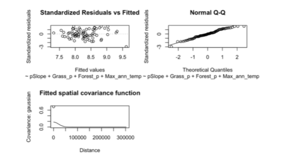
For initial data exploration and model selection efforts, we looked at spatial dependency using an empirical semivariogram. This analysis showed us interesting patterns of spatial correlation, with a nugget of about 0.5, a sill of 1.0, and a range of around 38,000 meters. We then used the Akaike Information Criterion (AIC) to find the best model for our analysis (we ultimately used AIC for all of our model performance evaluation). This involved adding variables one at a time and testing different types of spatial covariance—like exponential, Gaussian, spherical, Matérn, and none—to see which model explained fire size the best.

Our final model used Gaussian spatial linear regression, which helped us identify key factors affecting fire size. We found that maximum annual temperature and annual precipitation were significant predictors. Interestingly, higher temperatures were associated with smaller fire sizes, which suggests that extreme heat might not always lead to larger fires. Similarly, more precipitation was linked to smaller fires as well. While some factors like slope and population density weren't statistically significant, we kept them in the model to account for their potential influence.

We evaluated our model's fit using diagnostic plots, including a fitted vs. residuals plot and a Q-Q plot, both of which indicated that the model performed well and provided a reasonable fit to the data. The spatial covariance parameters from the final model—nugget (0.555), sill (0.174), and range (29,119 meters)—were not far from our initial estimates of nugget (~0.5), sill (~1.0), and range (~38,000 meters). This consistency suggests that our initial assumptions about spatial dependency were fairly accurate, further supporting the robustness of the model.

Once we had fit the model, we used it to predict fire sizes within the same location to get a sense of how it performs. The predictions tended to capture smaller fire sizes, which aligns with the observed data but also highlights some limitations in fully capturing the variability of larger fires. While this is not a perfect model, it represents a strong starting point for predicting fire sizes and understanding the factors that influence them. Future improvements could involve refining spatial covariance structures or incorporating additional variables to better account for larger fires and other complexities in fire behavior.

Point Process

Another way we approached the incidence data was utilization of the data attributes to subset fires by characteristics of incidence that we would like to study. We were primarily interested in IncidentSize, as previously discussed, and thresholding data to study large and small wildfire incidence as a point pattern realization. Further, we wanted to study differences in naturally occurring fires compared to human-caused, which we accomplished using the FireCause attribute. We analyzed different fire types at point processes using two different modeling approaches.

Log-Gaussian Cox Process Model

The Log-Gaussian Cox Process approach is used to determine the intensity surface of the response variable across the domain. For our application, we want to know the intensity of different types of wildfires across the domain of CC. The intensity at a location of $u$ is represented as $\lambda(u)$ where $\lambda(u)\sim N(0,C(\theta))$. There are a few options we could select for the covariance structure, but our data indicates that an exponential structure works best where $C(\theta)=C(u,u')=\sigma^2e^{-||u-u'||/h}$.

To fit this model, we need our predictor data to be grids of data points overlaying the entirety of CC that represent the intensity of each predictor. Due to computational limitations, it was only feasible to use a few data points for our prediction surfaces, so each point that we have corresponds to a large amount of land. This means that our predictors are not very granular and therefore the ability to predict the true intensity surface will be slightly diminished.

What we really care about is where future large wildfires might take place. If we have this information, we would be able to give a potential reason for the causes of wildfires and may be able to prevent them from occurring. Considering this, we wanted to look at where large wildfires exist and where small wildfires exist to be able to discern which areas are particularly at risk for large wildfires. This said, we believe that the type of wildfire, be it a natural or human caused one, largely impacts the cause and severity, so we decided to look at those two types of wildfires separately. Also, looking at the big picture, we wanted to see where all wildfires of each type would be occurring, so we looked at all, large and small wildfires for both natural and human caused wildfires, giving us six total response surfaces.

The code for formatting this data and running the models can be seen in Appendix B which yields the plots in Figure 4. Between natural and human caused, we can see a difference in regions of higher intensity. Natural wildfires occur both in the southern part and the northern part of CC, while human caused is predicted to occur in the southern part. We only have six large human caused wildfires, which means our intensity surface for those fires is uneventful, but form what we can see, it doesn't disagree with where the other sizes of human caused wildfires are. As for distinguishing where large natural wildfires tend to be compared to smaller ones, we don't really see much difference. It just seems that where there are a lot of wildfires, there are more chances for those wildfires to become bigger, so we see larger wildfires in the same areas as smaller wildfires.

The analysis of our intensity surfaces so far has been assuming that these models reflect our data well, but we should make sure this assumption is valid. For our covariance structure, the model fitting learns two parameters to make these surfaces which were the partial sill $\sigma^2$ and the range $h$.

From the table, we see that the maximum range is just below 30,000, which our units are in meters, so this is about 30km. This value is quite a bit larger than the second highest, but even the value of 30km is completely reasonable for this application. We do have issues with the partial sill parameter being essentially zero for large human caused wildfires, but this is easily explained by the fact that this model was fit to only 6 data points. The rest of the partial sill values are between 0.5 and 5, which are reasonable values to observe. Overall, we don't think that the range and sill parameters that we got from our models are alarming and this indicates that our choices for the model type and covariance structure are likely appropriate for this type of data. This leads us to look at how well our model is explaining our spatial structure.

The location of the wildfires could potentially be the result of a completely spatially random process, which would indicate that the model fitting approach that we are taking is not appropriate, so we created some envelope graphs to determine if our data points are completely spatially random, and if they aren't if our model is doing a good job at prediction.

The top row of these plots uses the $F(u,u')$ function while the bottom row used $G(u,u')$ and the green line represents the intercept only model and the red is our model. If all of these plots had the black lines within the envelope of the green lines, then we wouldn't have any evidence to suggest that our data points were not completely spatially random, but a few of the plots using $F(u,u')$ have their black line outside of the envelope giving us evidence that using modeling to find the intensity surface is a viable approach for this data set. Looking again at the plots using $F(u,u')$, we see that our model predicts the spatial intensity better than the intercept only for every size and type of wildfire, but the opposite is true when we look at $G(u,u')$. This leads us to believe that maybe we are using some predictors that are not important and are lacking some important predictors, humidity for example. After implementing the step function to our models to assess our model using AIC, which took a very long time, we got out the optimal model that strictly uses the intercept. This supports our thought that we should be using different predictors, but we don't believe that we should get rid of all the predictors that we are using. As mentioned previously, the data for this model's predictors were not very granular, which means the distance to roads is not very well captured. We still believe that is useful, but in future, if we use a higher resolution for our plots then some of these predictors may prove to be useful. Accompanying a higher resolution with other data points, we believe we could get a better intensity surface for our data which could give us some meaningful results about the effects of our predictors.

Binary Response GLM Logistic Regression Model

We wanted to hone in on large, naturally occurring wildfire incidence in CC in terms of risk spatially, and express that risk in probabilities of incidence for interpretable predictions. Evaluating spatial risk of this event can be valuable in prioritization of resources for mitigation efforts like thinning and prescribed burning for this unpredictable variety of wildfire incidence.

A binary response spatial GLM logistic regression model meets this criteria (see Appendix C). In order to build a binary response, we needed to supplement our incidence data with additional artificial data produced by a realization of a constant intensity $\lambda_0$ Poisson process. This data represents locations where large natural wildfires could have occurred but did not. We assigned a response $Y(\mathbf{s})=1$ to our real data and $Y(\mathbf{s})=0$ to the artificial data. The function spglm of the spmodel package was used to fit the model.

Similar to our other approaches, AIC was the chosen metric to objectively evaluate the performance of our model. Unfortunately, there is no R package that we could find to cycle our covariates for spglm objects in a manner similar to a function like stepAIC from the MASS package for lm objects. We built a loop to cycle different combinations of both predictors as well as spatial covariance fit functions. The lowest-AIC model we used for analysis used distance_rd_min_isprisec, a binary indicator variable describing whether the closest road was a major road or a remote road, $\log$ of population density, annual values for minimum temperature and precipitation as well as their interaction, and mean grass and forest densities as well as their interaction.

The lowest-AIC model used the wave spatial covariance function ($\sin(\eta)/\eta*\text{I}(h>0)+I(h=0),\,\,\eta=h/\text{range}, \,\,\, h=$ distance between observations). The intercept-only model with wave covariance fit performed fairly well with near-significance, indicating that the underlying processes influencing large wildfire incidence have some spatial trend. It should be noted that certain spatial covariance functions would cause the model fit to fail; the fixed effects were not converging, possibly due to using too small of a sample of points from the $\lambda_0$ process.

Our interpretation of a periodic spatial fit is that large wildfire incidence may be influenced by previous large wildfire incidence. The incidence describes the origin of the fire, which may spread in all directions, or primarily in one direction, and not many large fires could occur in its wake, creating a somewhat isotropic periodic pattern for large burns due to lack of fuel.

The model summary (see Appendix C) was in many ways underwhelming, and had identifiable shortcomings. Despite minimizing AIC, the final model did not return significance on any factors at the $\alpha=0.05$ level. This isn't necessarily concerning; a predictor is not required to be statistically significant at an arguably arbitrary threshold to be important to a model's prediction capability. However, it is at least of some concern that the confidence intervals of all fixed effects cover zero, and it is possible that our chosen covariates do not in fact influence the probability of large wildfire incidence meaningfully, but they at least surely do for our chosen performance metric. There were signs of some fixed effects that did not seem realistic, namely negative relationships for both annual minimum temperature and annual precipitation. Our model fit indicates that as we increase minimum annual temperature, or decrease annual precipitation, our probability of large wildfires actually goes down in general. There of course could be more than meets the eye here, but it certainly warrants further model investigation and possible refinements.

Our spatial covariance fit diagnostics returned results that are seemingly reasonable; $\sigma_{sill} = 2.832e+00$, $\sigma_{nugget} = 3.549e-02$, $\text{range} = 3.554e+04 \,\,(\sim\text{35.5 km})$. Namely, the range is something that is on a realistic scale at $\sim\text{35.5 km}$. Interpreting the range here is tricky, but we believe it could indicate a relationship with large fire incidence outside of some buffer region that could have to do with the area burned by that wildfire itself. We should also consider it may have to do with many other factors and be totally unrelated here, and that our domain in consideration is only CC, so this fit may only work best at this scale.

The predictions for our model were generated by creating a grid of evenly spaced points in CC (272 in total), and recovering the associated covariate data for these points on the last day of 2023 (to capture annual precipitation and temperature data for 2023). Using these points, we generated an incidence probability surface as included in Figure 7. Overlayed on this plot are the wildfire incidence points, as well as the outlines of the national forests in CC. The model favors higher probability of wildfire incidence in forested areas, especially within national forests, which is an intuitively realistic result. We take this as evidence that the model may have reasonable predictive capabilities, and has the advantage of having interpretable results.

Conclusions

We were able to successfully address each of our research questions with three different models that demonstrate proof-of-concept for our different approaches to the data. The covariate data that we selected did result in model improvements by AIC for most of our models, the only exception being for some of our LGCP fits. Evaluating CSR at different scales was an interesting exercise, and brought to light the importance of carefully selecting the spatial domain window for modeling efforts. There are some apparent shortcomings with each of our models, but we have identified paths forward for potential remedies to some issues we identified.

One of our challenges with covariates was somewhat self-inflicted. Our chosen covariates had some inefficiencies with recovering data for incidence observations, and there is a lesson to be taken away that it is important to be able to operate within a data framework that is accessible and manageable. It would be worthwhile to create rasters, or find other approaches, that would allow for faster recovery of covariate data. This would directly benefit the binary spatial GLM model, which is likely in need of generating more background process points for contrast in order for the point estimates of the fixed effects to stabilize.

Our chosen covariates improved our models by AIC, however there is much more to be studied and refined with their implementations. First, it's possible our environmental covariates could potentially be helping very little, if not hindering our models. There are of course interactions of countless environmental factors that influence the conditions that ultimately result in large wildfires. Part of the power of the spatial approach to statistical modeling is the ability to capture much of that information "qualitatively" with a spatial covariance fit. If environmental factors are introduced to a spatial model, we can introduce spatially confounding effects that may go undetected. A follow on effort should investigate further the question of how spatial confounding effects may impact these models.

Additionally, the inclusion of multiple environmental factors as predictors can introduce issues seen in vanilla statistical models like multicollinearity. Time did not permit a deeper dive into diagnostics and mitigation techniques for these undesirable effects, but it would certainly be worthwhile in any continued effort. Additional research might ask what other factors would be better to include, or in what other ways could a balance between spatial effects and other covariate data be achieved. We believe there may be some creative data available that could make meaningful improvements to our work, and we hope that inclusion of covariate data like distances to major or remote roads can serve as inspiration.

Lastly, one unexplored approach that we feel would be worthwhile for additional research is to attempt a spatio-temporal approach to modeling. Our models have only approached wildfire incidence spatially, but there is a temporal attribute to our data (FireDiscoveryDateTime) that could be utilized. Could temporal trends help to resolve some shortcomings of our models? Would we need the covariate data we studied, or would a spatio-temporal qualitative-only approach produce reasonable prediction models for wildfire size? These would be worthwhile explorations for anyone interested in this awesome dataset.

We believe that with some extra refinement, each model we produced could feasibly aid in better allocation of resources for fire prevention, possible forecasting, and information that could be coupled with other ecological models.

References