What Factors Affect My Free Throw Shot?

A Free Throw “Routine” Factor Screening

A Statistical Design of Experiments project

Background

For my Statistical Design of Experiments course final, I wanted to apply a statistical experiment to a sports problem, and specifically to one that might help improve my own game. I am an avid basketball fan, I play pick-up basketball from time to time, and I know that getting into games can often depend on simply making a free throw. My free throw technique was inconsistent, so honing in on some aspects that could help me shoot better was a constructive problem to tackle.

FreeThrow

The initial challenge in designing an experiment that could be worthwhile was determining what could be reasonably accomplished with limited resources. I was doing the project "solo", collecting only data about my own free throw shooting, and getting a large amount of data was essentially out of the question. I had a friend that would be able to help me out for a couple of hours on a weekend, which likely meant only getting one shot at getting an experiment run (we all have busy lives).

I had some intuition about a few technique factors that might be of interest, but no idea whether any of them would really affect my ability to shoot, for better or worse. So, it would be helpful to use a statistical experiment to determine if any of the factors that I had in mind really had any affect on how well I shoot free throws. This is how I landed on a $2^k$ factorial factor screening experimental design. If I am able to determine what factor(s) affect how I shoot, I can focus my efforts on improving that aspect of my technique.

$2^k$ Factorial Experiment Design

A $2^k$ Factorial design is useful here for some of its properties.

Can analyze multiple fixed factors of interest
- We can analyze different shooting techniques on their own
Factors can be qualitative
- The free throw shooting techniques are inherently qualitative
The design can account for nuisance factors
- There will be factors outside of the control of the experiments (location, wind, etc.)
Can be completely randomized
- We want to randomize our procedure
Describes the magnitude and direction for impact of factor(s) on the response
- While we are only performing a factor screening, it should indicate whether a particular techique positively or adversely affects shooting performance.

Factors selected for study

I spent some time thinking about how I approach free throw shooting, what techniques I had tweaked in the past, and ultimately decided upon the three different factors that I wanted to test.

Factor A: Time

Should I be taking my time before I shoot? Or is it better to shoot right away without thinking too much?

Factor B: Stance Angle

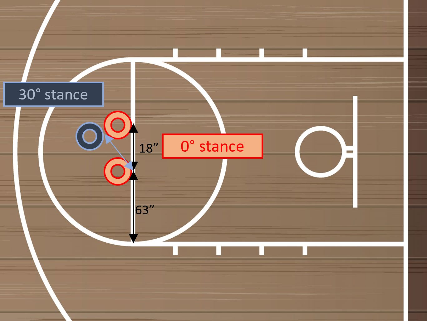
Should I stand with both toes touching the line, or at an angle?

Factor C: Spring

Does a "spring" motion (or lack of it) impact how well I shoot?

Factor "Levels"

The $2^k$ Factorial experimental design requires to test $k$ factors at two different levels each. One benefit of this design is the ability to use qualitative levels for our testing, which are described below.

	A	B	C
+	5 counts	~30° angle stance	"Spring" in legs
-	1 count	0° angle stance	"Stiff" legs

Procedures & Data Collection

Preparation

Worksheets
	Create worksheets for data collection to be recorded by assistant. Each worksheet has all $2^3$ combinations of factors sequenced in randomized order.

Stance Markings
	Mark foot positions on court with tape for repeatability of stance angle

15 minute warmup
Rehearsal of procedure with assistant

Procedure

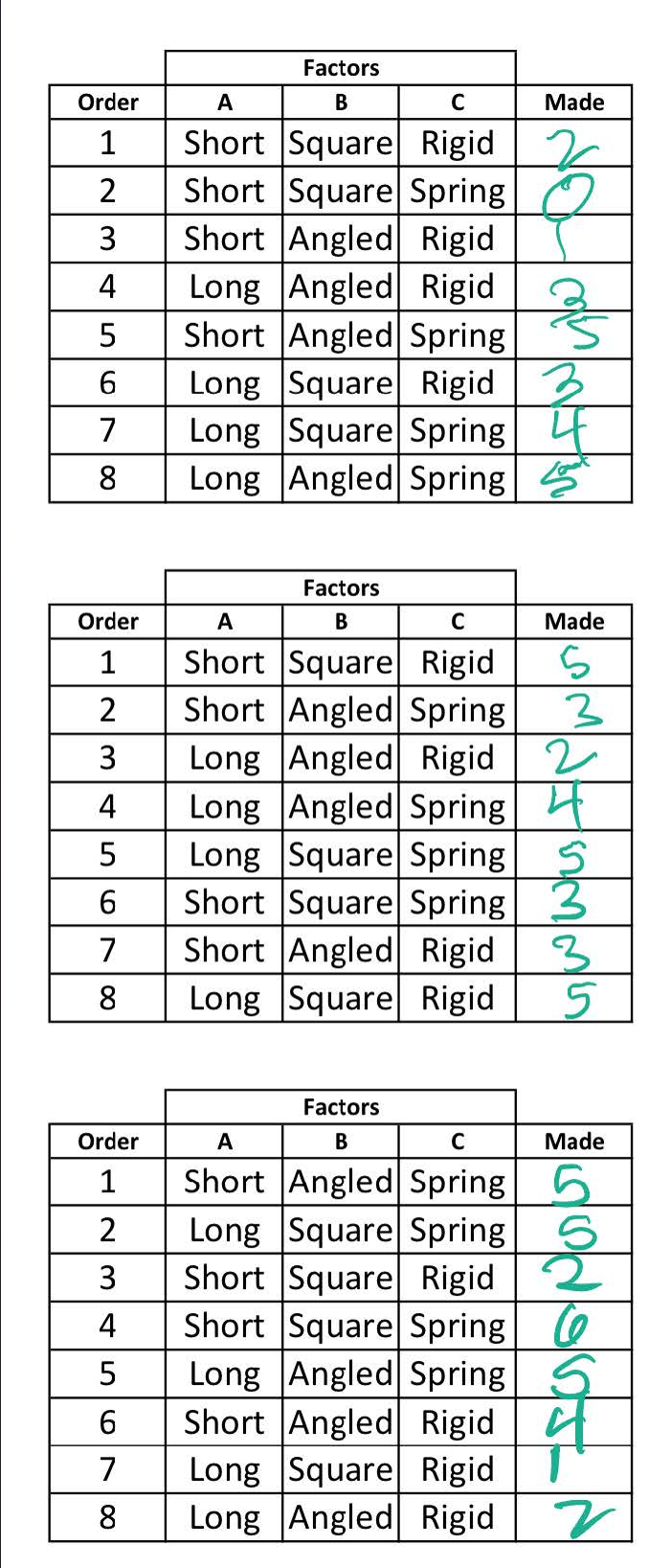
1 RUN (worksheet row)

Assistant announces factor combination for run, shooter adjusts stance angle
Assistant passes shooter ball, shooter dribbles for 1 or 5 counts and shoots rigid or with spring
Assistant retrieves ball, passes and process repeated until $X$ shots taken
Assistant records number made in run

Each of 8 runs (completely randomized) is performed to complete 1 replicate. As we will cover in the results, we uncovered some procedural issues in the data diagnostics (too few shots taken $X$ ), so an updated procedure was run in a new location. 3 replicates were performed at each location.

Statistical Model Details

$2^3$ Factorial Model

The model used for this experiment for the $2^{3}$ factorial model with blocked replicates is the following.

\begin{aligned} y_{ijkm}=A_{i}+B_{j}+C_{k}+(AB)_{ij}+(AC)_{ik}+(BC)_{jk}+(ABC)_{ijk}+\delta_{m}+\epsilon_{ijkm} \end{aligned}

$\begin{cases} i=1,2 \\ j=1,2 \\ k=1,2 \\ m=1,2 \end{cases}$

Hypothesis Testing

The hypotheses to be tested will be as follows.

\begin{aligned} H_{0} :A_{1}=A_{2}=0 \end{aligned}

\begin{aligned} H_{1} :\text{ at least one of } A_{1}\text{ or }A_{2}\neq0 \end{aligned}

And similar hypotheses for factors B and C.

\begin{aligned} H_{0} :(AB)_{ij}=0\,\,\text{ for all } i,j \end{aligned}

\begin{aligned} H_{1} :\text{at least one of }(AB)_{ij}\neq0 \end{aligned}

And similar hypotheses are extended for interactions $(AC)_{ik}$ , $(BC)_{jk}$ , and $(ABC)_{ijk}$ .

Model Assumptions

Factors are fixed (factors were selected and controlled in the experiment), so

\begin{aligned} A_{1}+A_{2}=0\text{, }B_{1}+B_{2}=0\text{, }C_{1}+C_{2}=0 \end{aligned}

\begin{aligned} \sum_{i=1}^{2}(AB)_{ij}=\sum_{j=1}^{2}(AB)_{ij}=0\text{, }\sum_{i=1}^{2}(AC)_{ik}=\sum_{k=1}^{2}(AC)_{ik}=0\text{, }\sum_{j=1}^{2}(BC)_{jk}=\sum_{k=1}^{2}(BC)_{jk}=0 \end{aligned}

\begin{aligned} \sum_{i=1}^{2}(ABC)_{ijk}=\sum_{j=1}^{2}(ABC)_{ijk}=\sum_{k=1}^{2}(ABC)_{ijk}=0 \end{aligned}

and error is normally distributed

\begin{aligned} \epsilon_{ijkm}\sim N(0,\sigma^{2}) \end{aligned}

Design Matrix

	A	B	C
$r_1$	-	-	-
$r_2$	+	-	-
$r_3$	-	+	-
$r_4$	+	+	-
$r_5$	-	-	+
$r_6$	+	-	+
$r_7$	-	+	+
$r_8$	+	+	+

Results

Notes about experiments

Locations

In total, this experiment was carried out at 3 different locations. One location was an indoor court, the other two were two different outdoor courts. One of the inherent advantages of this design is that it can deal well with nusiance factors. Even though each location may have its own nusance factors (for example, it may be windy outdoors), the datasets that were collected were all contained within their own experimental runs. So, since we are contrasting factors within each experiment (and not comparing experiments to each other), any noise introduced to the system by nusiance factors should be contained within each individual experiment and thus should not impact comparisons. If there is disruption, we should be able to detect with data normality diagnostics.

Normality diagnostics

The first two experiments, Indoor I and Outdoor I, were performed prior to any data analysis being executed. When a cursory analysis was performed, there was an issue identified. The normality diagnostics, namely the Shapiro-Wilk and Anderson-Darling normality measures indicated that our normality assumptions for both the Indoor I and Outdoor I data were borderline at best. Further, the results indicated a significant ( $\alpha=0.05$ level) third-order interaction between factors for the Indoor I experiment, and similar borderline significant third order interactions for the Outdoor I experiment. The result was isolated to the third-order interactions; all other terms were not indicating significance.

Sample Size

The isolated third-order significance and borderline normality assumptions can be indicative of issues with sample size. For each of the first two experiments, $X=5$ shots were taken at each factor combination run. It was worthwhile for the sake of the integrity of the experiment to rerun with a greater sample size with hopes of increasing the fidelity.

For the Outdoor II experiment, $X=10$ shots were taken for each factor combination run. This proved effective; all normality diagnostics cleaned up, and we found significance at an $\alpha=0.05$ level for one of our factors, which we will discuss next.

Indoor I Results

Outdoor I Results

Outdoor II Results

Conclusions

Inference

Factor C (Spring/Rigid) is approximately significant at the $\alpha=0.05$ level in Outdoor II factor screening experiment
Factor C has a positive effect on response from low level to high level (Rigid to Spring) for the Outdoor II factor screening experiment

Caveats

Can only infer about fixed factors, and results are valid only for specific locations and conditions.
- Our results technically only apply to the specific conditions of each factor we tested, and how they were specifically carried out within the experiment. However, it is still a useful first step to determine what factors may generally be important, and which ones are probably worth disregarding.
Study only “screens” for factor of interest.
- We cannot reasonably take away any quantitative results of the impacts of Factor C as truth. Rather, we can only infer that using the "Spring" motion improves my shooting ability for these conditions. However, it is useful to know that it actually improves my shot to use the motion, and it could become the subject of an experiment investigating that factor in greater detail.

Lessons Learned

Larger sample size, repeated experiments; proper power analysis may be warranted.
Unplanned nuisance factors may have impacted the experiment. Fatigue, for example, should be considered as the experiment progresses.

Further Study

Focused study on “Spring” factor effects, new experimental design
Factor screening of additional subjects

Bibliography

Fazel, F., Morris, T., Watt, A., & Maher, R. (2018). The effects of different types of imagery delivery on basketball free-throw shooting performance and self-efficacy. Psychology of Sport and Exercise, 39, 29–37. https://doi.org/https://doi.org/10.1016/j.psychsport.2018.07.006

May, A. J. (2011). A Comparison of the Effectiveness of Two Free Throw Shooting Methods. https://api.semanticscholar.org/CorpusID:142202085

Montgomery, D. C. (2012). Design and Analysis of Experiments, 8th Edition. John Wiley & Sons, Incorporated. https://books.google.com/books?id=XQAcAAAAQBAJ

Reproducibility

Paper

Final Paper

Data

Link to datasets

SAS code

/* Indoor Factorial 2023 APR 15 */
/* SELECT DATA */
/* alexfactorial20230415 . xlsx */
/* alexfactorialoutdoor20230422 . xlsx */
/* alexfactorialoutdoor20230425 . xlsx */
proc import datafile ="/ home /.../ alexfactorialoutdoor20230425 . xlsx "
dbms = xlsx
out = alexf1
replace ;
getnames = yes ;
run ;
data inter ;
set alexf1 ;
AB=A*B;
AC=A*C;
BC=B*C;
ABC =A*BC;
block = Run ;
resp = of5made ;
proc glm data = inter ;
class A B C AB AC BC ABC block ;
model resp = block A B C AB AC BC ABC ;
output out = diag r=res p= pred ;
run ;
/* check normality */
proc univariate data = diag normal ;
var res ;
qqplot res / normal (mu= est sigma = est );
run ;
/* check constant variance using graph */
title 'residual plot : res vs predicted value ';
proc sgplot data = diag ;
scatter x= pred y=res;
refline 0;
run ;
proc reg data = inter ;
model resp = block A B C AB AC BC ABC ;
run ;
/* FIT MODEL TO ONLY FACTOR C */
proc glm data = inter ;
class A B C AB AC BC ABC block ;
model resp = block C;
output out = diag r=res p= pred ;
run ;
/* check normality */
proc univariate data = diag normal ;
var res ;
qqplot res / normal (mu= est sigma = est );
run ;
/* check constant variance using graph */
title 'residual plot : res vs predicted value ';
proc sgplot data = diag ;
scatter x= pred y=res;
refline 0;
run ;
proc reg data = inter ;
model resp = block C;
run ;

Statistical Design Of Experiments